学生时代,其实事情就那么多,做完作业,或者完成阶段性成果,就i可以玩儿了。所以,我养成了快速完成,经常加班的习惯,因为加班了,后面就是一段假期。
但工作后,情况不一样了,事情是做不完的,一件事情完了还有一件事情,但还是高强度的工作,身体有时候是吃不消的。
回头,还是严格遵守,工作时间完成工作,下班后,不要再加班了。
工作,和生活,一定要学会分开,不要搅在一起。
学生时代,其实事情就那么多,做完作业,或者完成阶段性成果,就i可以玩儿了。所以,我养成了快速完成,经常加班的习惯,因为加班了,后面就是一段假期。
但工作后,情况不一样了,事情是做不完的,一件事情完了还有一件事情,但还是高强度的工作,身体有时候是吃不消的。
回头,还是严格遵守,工作时间完成工作,下班后,不要再加班了。
工作,和生活,一定要学会分开,不要搅在一起。
# -*- coding: utf-8 -*-
"""
Created on Wed Sep 17 15:37:16 2025

@author: cdlei
"""


import backtrader as bt
import pandas as pd


symbol='515800'

def read_data(symbol):
    file="./data/"+symbol+".csv"
    daily_price = pd.read_csv(file,parse_dates=['date'])
    data=daily_price.set_index('date')
    return data


class TestStrategy(bt.Strategy):


    params=(('period1',5),
           ('period2',10),)

    def log(self, txt, dt=None):
       ''' Logging function fot this strategy'''
       dt = dt or self.datas[0].datetime.date(0)
       print('%s, %s' % (dt.isoformat(), txt))

    def __init__(self):
        # 打印数据集和数据集对应的名称


        # print("-------------self.datas-------------")
        # print(self.datas)
        # print("-------------self.data-------------")
        # print(self.data._name, self.data)
        # print("-------------self.data0-------------")
        # print(self.data0._name, self.data0)
        # print("-------------self.datas[0]-------------")
        # print(self.datas[0]._name, self.datas[0])

        # print(self.data.close)
        # print(self.data.open)

        #计算均线

        self.ma1 = bt.indicators.SMA(self.data.close, period=self.p.period1)
        self.ma2 = bt.indicators.SMA(self.data.close, period=self.p.period2)

        #计算2条均线交叉信号:ma2 上穿 ma1 时,取值为 +1; ma2 下穿 ma1 时,取值为 -1
        self.crossover = bt.indicators.CrossOver(self.ma2, self.ma1)
        # 初始化订单
        self.order = None

    def next(self):


        # 打印每日的资金和持仓情况
        print('date', self.data0.datetime.date(0))
        print('当前可用资金', self.broker.getcash())
        print('当前总资产', self.broker.getvalue())
        print('当前持仓量', self.broker.getposition(self.data).size)
        print('当前持仓成本', self.broker.getposition(self.data).price)

        # 取消之前未执行的订单
        if self.order:
            self.cancel(self.order)


        # 检查是否有持仓
        if not self.position:
            # 10日均线上穿5日均线,买入
            if self.crossover > 0:
                self.order = self.buy(size=10000) # 以下一日开盘价买入10000股
        # # 10日均线下穿5日均线,卖出
        elif self.crossover < 0:
            self.order = self.close() # 平仓,以下一日开盘价卖出

    def notify_order(self, order):
        # 未被处理的订单
        if order.status in [order.Submitted, order.Accepted]:
            return
        # 已被处理的订单
        if order.status in [order.Completed, order.Canceled, order.Margin]:
            if order.isbuy():
                self.log(
                    '执行买入, ref:%.0f,Price: %.4f, Size: %.2f, Cost: %.4f, Comm %.4f, Stock: %s' %
                    (order.ref,
                     order.executed.price,
                     order.executed.size,
                     order.executed.value,
                     order.executed.comm,
                     order.data._name))
            else:  # Sell
                self.log('执行卖出, ref:%.0f, Price: %.4f, Size: %.2f, Cost: %.4f, Comm %.4f, Stock: %s' %
                        (order.ref,
                        order.executed.price,
                         order.executed.size,
                        order.executed.value,
                        order.executed.comm,
                        order.data._name))


#使用示例

if __name__ == '__main__':

    #读取数据
    data=read_data(symbol)
    #修改格式
    datafeed = bt.feeds.PandasData(dataname=data)
    cerebro=bt.Cerebro()
    #添加策略
    cerebro.addstrategy(TestStrategy)
    #加载数据
    cerebro.adddata(datafeed)
    #设置初始资金
    cerebro.broker.set_cash(100000)

    #设置滑点
    #cerebro.broker.set_slippage_perc(perc=0.0001)

    #运行回测
    cerebro.run()

    #输出最终资产
    print(f'最终资产价值:{cerebro.broker.getvalue():.2f}')
近期,事情有点多,家里事情也多,好好调整下状态。
明天,应该可以进入 运动+学习+工作的节奏了。
hapyy new term!
明天开始继续搞量化了。
半天量化+半天艺术。
转自微信公众号 《数据科学实战》
import numpy as np

# 从 Python 列表创建
price_list = [143.73, 145.83, 143.68, 144.02, 143.5, 142.62]
price_array = np.array(price_list)
print(f"一维数组:{price_array}")

# 从列表的列表创建二维数组(矩阵)
ohlc_data = np.array([[143.73, 145.90, 143.50, 145.83],
                      [145.83, 146.20, 143.68, 143.68]])
print(f"\n二维数组(矩阵):\n{ohlc_data}")

# 专用数组创建函数
zeros_array = np.zeros(5)  # 5个零的数组
ones_matrix = np.ones((2, 3))  # 2x3的全1矩阵
price_range = np.linspace(100, 110, 11)  # 100到110之间均匀分布的11个点
random_returns = np.random.randn(10)  # 10个来自标准正态分布的随机数

print(f"\n全零数组:{zeros_array}")
print(f"\n全一矩阵:\n{ones_matrix}")
print(f"\n线性间隔数组:{price_range}")
print(f"\n模拟随机收益率:{random_returns}")

import time

# 模拟一个包含5000个资产的大型投资组合
num_assets = 5000

# 生成随机权重(总和为1)
weights = np.random.random(num_assets)
weights /= np.sum(weights)

# 为每个资产生成随机收益率
returns = np.random.randn(num_assets) * 0.01  # 小的日收益率

# --- 方法1:Python 循环 ---
start_time_loop = time.time()
portfolio_return_loop = 0.0
for i in range(num_assets):
    portfolio_return_loop += weights[i] * returns[i]
end_time_loop = time.time()
time_loop = (end_time_loop - start_time_loop) * 1000  # 毫秒

print(f"投资组合收益率(循环法):{portfolio_return_loop:.6f}")
print(f"耗时(循环法):{time_loop:.4f} 毫秒")

# --- 方法2:NumPy 向量化点积 ---
start_time_np = time.time()
portfolio_return_np = np.dot(weights, returns)
end_time_np = time.time()
time_np = (end_time_np - start_time_np) * 1000  # 毫秒

print(f"\n投资组合收益率(NumPy法):{portfolio_return_np:.6f}")
print(f"耗时(NumPy法):{time_np:.4f} 毫秒")

# --- 性能比较 ---
print(f"\nNumPy 方法大约比循环快 {time_loop/time_np:.0f} 倍。")


pip install numpy-financial

import numpy_financial as npf

# 示例:计算项目的净现值(NPV)
# 一个项目需要10万美元的初始投资
# 预计在4年内产生3万、4万、5万和6万美元的现金流
# 折现率为8%
rate = 0.08
cash_flows = np.array([-100000, 30000, 40000, 50000, 60000])

# npv函数计算未来现金流的净现值(从第1年开始)
# 所以我们计算后再加上初始投资
net_present_value = npf.npv(rate, cash_flows[1:]) + cash_flows[0]
print(f"项目现金流:{cash_flows}")
print(f"折现率:{rate:.2%}")
print(f"净现值(NPV):${net_present_value:,.2f}")

# 示例:计算内部收益率(IRR)
internal_rate_of_return = npf.irr(cash_flows)
print(f"内部收益率(IRR):{internal_rate_of_return:.2%}")

import pandas as pd

# 创建股票价格的 Series
aapl_prices = pd.Series([171.5, 172.3, 170.9, 173.1],
                        index=['2023-11-01', '2023-11-02', '2023-11-03', '2023-11-04'])
print("Pandas Series:")
print(aapl_prices)
print(f"\n2023-11-02 的价格:{aapl_prices['2023-11-02']}")

# 从字典创建 DataFrame
data = {'Open': [171.5, 172.3, 170.9, 173.1],
        'High': [172.8, 173.5, 171.2, 174.0],
        'Low': [170.1, 171.8, 170.5, 172.5],
        'Close': [172.3, 170.9, 173.1, 173.9],
        'Volume': [5.2e7, 4.8e7, 5.5e7, 4.9e7]}

dates = pd.to_datetime(['2023-11-01', '2023-11-02', '2023-11-03', '2023-11-04'])
df = pd.DataFrame(data, index=dates)

print("\nPandas DataFrame:")
print(df)

# 通过标签(日期)选择单行
print("\n使用 .loc 获取 2023-11-02 的数据:")
print(df.loc['2023-11-02'])

# 通过行列标签选择单个值
close_price = df.loc['2023-11-03', 'Close']
print(f"\n2023-11-03 的收盘价:{close_price}")

# 选择行和特定列的切片
print("\n使用 .loc 选择行和列的切片:")
print(df.loc['2023-11-02':'2023-11-04', ['Open', 'Close']])

# 选择第一行(索引为0)
print("\n使用 .iloc 获取第一行数据:")
print(df.iloc[0])

# 选择第3行、第4列的值(索引均为3)
volume_val = df.iloc[3, 4]
print(f"\n第4天的成交量:{volume_val}")

# 选择第1行和第2行,以及第0列和第3列
print("\n使用 .iloc 选择行和列的切片:")
print(df.iloc[1:3, [0, 3]])

# 找出所有收盘价高于172的日子
high_close_days = df[df['Close'] > 172]
print("\n收盘价 > 172 的日子:")
print(high_close_days)

# 组合多个条件:找出成交量高且价格区间大的日子
high_volume_threshold = 5.0e7
large_range_threshold = 2.0
active_days = df[(df['Volume'] > high_volume_threshold) &
                ((df['High'] - df['Low']) > large_range_threshold)]
print("\n高成交量、大价格区间的日子:")
print(active_days)
转自微信公众号 《数据科学实践》
# 交易示例
number_of_shares = 100
trade_id = 15432
days_to_expiry = 30
print(f"Trade ID {trade_id}: Bought {number_of_shares} shares.")
print(f"Type of 'number_of_shares': {type(number_of_shares)}")

# 金融指标示例
stock_price = 149.95
interest_rate = 0.0525  # 5.25% 的利率
daily_return = -0.015   # -1.5% 的日收益率
print(f"Current stock price: ${stock_price}")
print(f"Type of 'stock_price': {type(stock_price)}")

#浮点精度问题
val = 0.35 + 0.1
print(val)  # 输出: 0.44999999999999996


#使用Decimal模块
from decimal import Decimal
# 使用 Decimal 进行精确的金融计算
fee_1 = Decimal('0.35')
fee_2 = Decimal('0.10')
total_fee = fee_1 + fee_2
print(f"Total fee with Decimal: {total_fee}")  # 输出: 0.45

# 资产标识符示例
ticker = 'aapl'
currency_pair = 'EURUSD'
sector = 'Information Technology'
# 使用字符串方法标准化数据
standardized_ticker = ticker.upper()  # 常见做法
print(f"Standardized Ticker: {standardized_ticker}")
# F-字符串可用于创建格式化报告
trade_confirmation = f"Executed trade for 100 shares of {standardized_ticker}"
print(trade_confirmation)

# 交易系统中的标志示例
is_market_open = True
has_sufficient_capital = True
is_trade_profitable = (151.25 - stock_price) > 0  # 这个表达式会计算为布尔值
# 布尔值控制决策
if is_market_open and has_sufficient_capital:
    print("System is ready to place a trade.")
else:
    print("System is offline or capital is insufficient.")
print(f"Is the trade profitable? {is_trade_profitable}")


#**列表 (list)**:可变、有序的元素序列,用于存储历史价格时间序列或交易记录集合:
# 一周的股票收盘价示例
aapl_prices_list = [150.10, 151.20, 150.85, 152.50, 152.30]
aapl_prices_list.append(153.10)  # 列表是可变的,可以添加元素
print(f"Price on the first day: {aapl_prices_list[0]}")
print(f"Updated price list: {aapl_prices_list}")

#**元组 (tuple)**:不可变、有序的序列。在金融中,许多记录一旦创建就应永久保存:
# 已完成的交易记录示例
trade_record = ('AAPL', 152.50, 100, '2023-10-27T10:00:00Z')
# 尝试修改它会引发错误,确保数据完整性
# trade_record[1] = 152.60  # 这会引起 TypeError
print(f"Immutable Trade Record: {trade_record}")

# 简单股票投资组合示例
portfolio = {'AAPL': 100, 'GOOG': 50, 'MSFT': 75}
# 访问持仓
print(f"Shares of GOOG held: {portfolio['GOOG']}")
# 添加新持仓
portfolio['AMZN'] = 25
print(f"Updated Portfolio: {portfolio}")
# 更新现有持仓
portfolio['AAPL'] += 50  # 又买了 50 股
print(f"Final shares of AAPL: {portfolio['AAPL']}")

# 管理观察清单示例
watchlist_1 = {'AAPL', 'MSFT', 'GOOG', 'AMZN'}
watchlist_2 = {'AAPL', 'NVDA', 'TSLA', 'MSFT'}
# 查找两个观察清单中的共同股票(交集)
common_stocks = watchlist_1.intersection(watchlist_2)
print(f"Common Stocks: {common_stocks}")
# 查找两个观察清单中的所有唯一股票(并集)
all_stocks = watchlist_1.union(watchlist_2)
print(f"All Unique Stocks: {all_stocks}")

# 简化的价格数据示例
prices = [5, 6, 7, 7, 6, 9, 8, 9, 9, 7, 6, 6]
# 本例中使用简化的"当前"移动平均线
# 实际场景中,这些会基于完整历史计算
short_term_sma = sum(prices[-3:]) / 3  # 3 天 SMA
long_term_sma = sum(prices[-7:]) / 7   # 7 天 SMA
print(f"Short-term SMA: {short_term_sma:.2f}")
print(f"Long-term SMA: {long_term_sma:.2f}")
# 使用条件语句实现交易逻辑
if short_term_sma > long_term_sma:
    print("Signal: BUY")
    print("Reason: Short-term momentum is positive.")
elif short_term_sma < long_term_sma:
    print("Signal: SELL")
    print("Reason: Short-term momentum is negative.")
else:
    print("Signal: HOLD")
    print("Reason: No clear trend divergence.")

tickers = ['AAPL', 'MSFT', 'GOOG', 'AMZN']
print("Processing trades for the following tickers:")
for ticker in tickers:
    # 实际应用中,这里会调用数据获取函数
    print(f" -> Fetching latest price for {ticker}...")
    # 模拟一些处理过程
    print(f" -> Analyzing {ticker} for trading opportunities.")

portfolio = {'AAPL': 150, 'NVDA': 50, 'TSLA': 75}
# 假设我们已将最新价格获取到另一个字典中
current_prices = {'AAPL': 171.50, 'NVDA': 460.18, 'TSLA': 256.49}
total_portfolio_value = 0.0
print("\nCalculating portfolio value:")
for ticker, shares in portfolio.items():
    price = current_prices[ticker]
    position_value = shares * price
    total_portfolio_value += position_value
    print(f" Position: {ticker}, Shares: {shares}, Value: ${position_value:,.2f}")
print(f"\nTotal Portfolio Market Value: ${total_portfolio_value:,.2f}")

import random
# 简化的风险值示例
# 实际中,这会是复杂计算,如投资组合标准差
asset_risks = {'Bonds': 0.05, 'BlueChipStock': 0.15, 'TechStock': 0.25, 'Crypto': 0.40}
asset_list = list(asset_risks.keys())
max_portfolio_risk = 0.50
current_portfolio_risk = 0.0
portfolio_composition = []
print(f"\nBuilding portfolio with max risk target of {max_portfolio_risk:.2f}:")
# 只要风险低于最大值就继续添加资产
while current_portfolio_risk < max_portfolio_risk:
    # 随机选择要添加的资产
    asset_to_add = random.choice(asset_list)
    asset_risk_value = asset_risks[asset_to_add]
    # 检查添加此资产是否会超过最大风险
    if current_portfolio_risk + asset_risk_value > max_portfolio_risk:
        print(f"Cannot add {asset_to_add} (risk {asset_risk_value:.2f}), would exceed max risk.")
        break  # break 语句立即退出循环
    # 添加资产并更新风险
    portfolio_composition.append(asset_to_add)
    current_portfolio_risk += asset_risk_value
    print(f" Added {asset_to_add}. Current portfolio risk: {current_portfolio_risk:.2f}")
print(f"\nFinal Portfolio Composition: {portfolio_composition}")
print(f"Final Portfolio Risk: {current_portfolio_risk:.2f}")


def function_name(parameter1, parameter2):
    """
    这是文档字符串。它解释函数的功能。
    专业代码必须有良好的文档字符串。
    """
    # 执行操作的代码块
    result = parameter1 + parameter2
    return result

import math
def calculate_annualized_volatility(prices_list):
    """
    从日价格列表计算股票的年化波动率。

    参数:
    prices_list (list): 表示日价格的浮点数或整数列表

    返回:
    float: 年化波动率
    """
    # 步骤 1: 计算日收益率
    daily_returns = []
    for i in range(1, len(prices_list)):
        # (今日价格 / 昨日价格) - 1
        daily_return = (prices_list[i] / prices_list[i-1]) - 1
        daily_returns.append(daily_return)

    if not daily_returns:
        return 0.0

    # 步骤 2: 计算收益率的标准差
    # 首先,计算平均收益率
    mean_return = sum(daily_returns) / len(daily_returns)
    # 然后,计算方差
    variance = sum([(r - mean_return) ** 2 for r in daily_returns]) / len(daily_returns)
    std_dev = math.sqrt(variance)

    # 步骤 3: 将波动率年化
    trading_days = 252
    annualized_volatility = std_dev * math.sqrt(trading_days)

    return annualized_volatility

# --- 使用函数 ---
aapl_prices = [150.1, 151.2, 150.8, 152.5, 152.3, 153.1, 155.0, 154.5]
volatility = calculate_annualized_volatility(aapl_prices)
print(f"Calculated Annualized Volatility: {volatility:.2%}")

# 导入整个模块
import math
print(math.sqrt(25))  # 使用 module_name.function_name 调用函数

# 从模块导入特定函数
from math import sqrt
print(sqrt(25))  # 直接按名称调用函数

# 量化社区通用约定是使用别名
import numpy as np
import pandas as pd
import matplotlib.pyplot as plt


###
#创建模块文件:在项目目录中创建名为 financial_metrics.py 的新文件。

#向模块添加函数:

###

import math

def calculate_annualized_volatility(prices_list):
    """
    从日价格列表计算股票的年化波动率。
    ... (与前面相同的文档字符串)...
    """
    #... (与前面相同的函数代码)...
    return annualized_volatility

def calculate_simple_return(start_price, end_price):
    """计算一段时间内的简单收益率。"""
    return (end_price / start_price) - 1

#导入和使用自定义模块:
# 导入自定义模块
import financial_metrics

# 使用模块中的函数
aapl_prices = [150.1, 151.2, 150.8, 152.5, 152.3, 153.1, 155.0, 154.5]
vol = financial_metrics.calculate_annualized_volatility(aapl_prices)
ret = financial_metrics.calculate_simple_return(aapl_prices[0], aapl_prices[-1])
print(f"Using our custom module:")
print(f" Annualized Volatility: {vol:.2%}")
print(f" Total Return: {ret:.2%}")
转自微信公众号 《数据科学与实战》
1、获取历史股票数据
2、计算移动平均线等技术指标
3、可视化股价走势
4、计算关键风险回报指标(如夏普比率)
5、分析回报率分布
import numpy as np
import pandas as pd
import matplotlib.pyplot as plt
import yfinance as yf
from datetime import datetime, timedelta

# 设置时间范围(过去一年)
end_date = datetime.now()
start_date = end_date - timedelta(days=365)

# 下载股票数据(以阿里巴巴为例)
ticker = "BABA"
stock_data = yf.download(ticker, start=start_date, end=end_date)

# 查看数据的前几行
print(f"{ticker} 股票数据概览:")
print(stock_data.head())

# 计算简单的技术指标 - 20日和50日移动平均线
stock_data['MA20'] = stock_data['Close'].rolling(window=20).mean()
stock_data['MA50'] = stock_data['Close'].rolling(window=50).mean()

# 绘制股票价格和移动平均线
plt.figure(figsize=(12, 6))
plt.plot(stock_data.index, stock_data['Close'], label='收盘价', color='blue')
plt.plot(stock_data.index, stock_data['MA20'], label='20日均线', color='red')
plt.plot(stock_data.index, stock_data['MA50'], label='50日均线', color='green')
plt.title(f'{ticker} 过去一年股价走势及移动平均线')
plt.xlabel('日期')
plt.ylabel('价格(美元)')
plt.legend()
plt.grid(True, alpha=0.3)
plt.show()

# 计算每日回报率
stock_data['Daily_Return'] = stock_data['Close'].pct_change() * 100

# 计算基本统计数据
mean_return = stock_data['Daily_Return'].mean()
std_return = stock_data['Daily_Return'].std()
annual_return = mean_return * 252  # 假设一年有252个交易日
annual_volatility = std_return * np.sqrt(252)
sharpe_ratio = annual_return / annual_volatility  # 假设无风险利率为0

print(f"\n{ticker} 基本统计数据:")
print(f"平均日回报率: {mean_return:.2f}%")
print(f"回报率标准差: {std_return:.2f}%")
print(f"年化回报率: {annual_return:.2f}%")
print(f"年化波动率: {annual_volatility:.2f}%")
print(f"夏普比率: {sharpe_ratio:.2f}")

# 绘制回报率分布直方图
plt.figure(figsize=(10, 6))
plt.hist(stock_data['Daily_Return'].dropna(), bins=50, alpha=0.75, color='blue')
plt.axvline(0, color='red', linestyle='--', linewidth=1)
plt.title(f'{ticker} 日回报率分布')
plt.xlabel('日回报率 (%)')
plt.ylabel('频率')
plt.grid(True, alpha=0.3)
plt.show()
本来开始想用云服务器发短信功能。但后面考虑两个问题:
需要企业备案和短信包要花钱。
最后采用钉钉机器人的方式,初步解决了问题。
下一步: 实时跟踪ETF基金分钟行情,设计跟踪信号。然后发送到钉钉群提醒。
微信群用于工作,钉钉群用于接收行情信号提醒。挺好的。
看后面能否稳定运行。
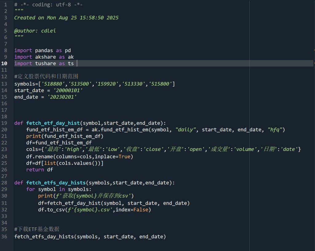
Akshare, Tushare,获取日线数据,可以。
但分钟线,akshare接口失效,tushare价格昂贵。
最后,还是决定自己写个爬虫程序。
花了一天,终于搞定。
跟踪几个小标的,应该问题不大。
希望后面不被封掉。
封了的话,再看是否需要IP代理。
前前后后做了很多的铺垫,一直没有真正投入精力去做这个事情。今年行情不错,可能接近行情尾声了。
但,一直想做的量化交易,还是需要抽空给搭建起来。
先把实时盯盘程序完成吧。看一个星期能不能搞定。
先不忙动交易的事情。先机器人盯盘。